
Written by: Marc Odo | Swan Global Investments
Why Investors Should Listen to Hall of Famer Ken Griffey. Jr
Consistency of returns is an important driver of overall investment results, just like in sports and other areas of our lives. In fact, investors and advisors could learn a lot from the intentional consistency sought after by top sports performers.
Consistency Is King, Both in Sports and Investing
On July 24, 2016, the greatest ballplayer I’ve ever seen was inducted in the National Baseball Hall of Fame with a record-setting 99.3% of the vote. Reflecting on his career, Ken Griffey, Jr. recently said:
“On the Mariners, we had this philosophy in the clubhouse that we referred to as Baseball Gods. Maybe it was more of a superstition than a philosophy. When someone referred to Baseball Gods, we were acknowledging that this game will make you feel human really fast: Never get too high on yourself and never get too low. It was a reminder that you’re never as bad as they say you are and never as good as you think you are.”
What Griffey said about baseball can also be said about the markets: They always have a way of humbling you. It’s important to keep your head on straight when markets are either soaring or crashing.
Unfortunately, that’s easier said than done given the wild ride the markets have been on over the last decade or two. The graph below shows a breakout of annualized returns for every three-year period between July 1,1997 to December 31, 2019.
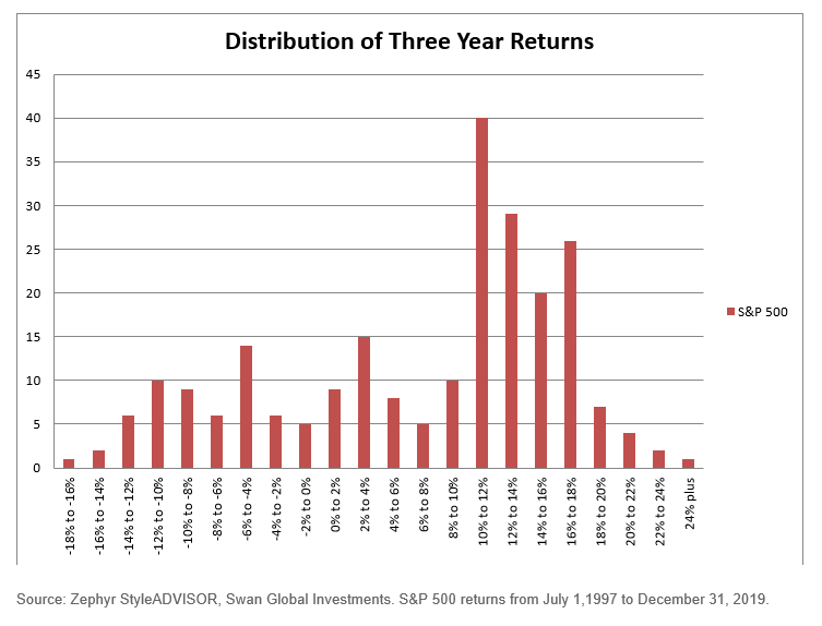
Return Distribution: A Test of Consistency
A plain English description of this distribution might be “feast or famine.” The more formal, statistical description is that this is a bi-modal distribution.
Usually a distribution will be clustered near the mean, or average result, and then gently slope off in both directions.
However, this distribution has two or maybe even three peaks (tri-modal). A large number of occurrences cluster in 10%-to-18% range, which represents a very healthy return.
In addition, there are also many occurrences where the annualized three-year returns were in the -8% to -14% range. Even more interesting, while the average three-year annualized return for the S&P 500 is 6.83%, there are very few times since July 1997 that the S&P 500 was close to its average—it was typically either way above or way below.
A similar, bi-modal distribution appears when looking at long-term, ten-year annualized returns. The largest bucket representing 39.1% of the outcomes is the 6% to 8% range; a perfectly acceptable result for most investors.
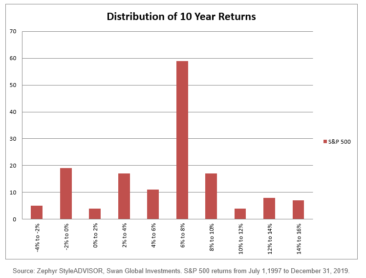
Worryingly though, the second most frequent range of ten-year returns is actually negative, ranging from -2% to 0%. Combined with the -4% to -2% bucket, 15.9% of the observations in this range were “lost decades.”
Seeking Narrow Distribution or Return Consistency
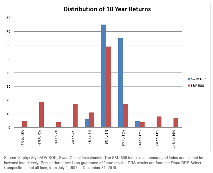
The Defined Risk Strategy (DRS) was designed to mitigate the impact of these outlier events and possibly provide a smoother, more reliable, more consistent outcome. By actively hedging against bear markets, the DRS has a much smaller “left tail” of bad outcomes. Over its 20-year history, the DRS Select Composite has weathered the two largest bear markets since World War II: the dot-com bust of 2000-2002 and the financial crisis of 2007-09. Below we see the distribution of annualized three-year returns of the DRS Select Composite compared to the S&P 500.
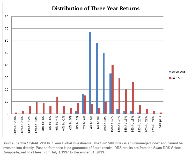
By hedging with long-term put options, the DRS Select Composite has historically minimized the impact of those bear markets. The distribution of DRS returns is what one hopes to see—the majority of returns are clustered near the average of the distribution.
The long-term returns of the DRS Select Composite are much more predictable. There isn’t a second peak to the distribution out in negative territory like there is for the S&P 500.
Of course, by maintaining the hedge at all times, the DRS will lag in up markets. There will be fewer observations in the high-teens or over -20% range. However, that is a trade-off the DRS Select Composite has willingly accepted. It has always been Swan’s philosophy that avoiding losses is more important than capturing all of the market’s gains.
The logic and justification for this are spelled out in our white paper “Math Matters: Rethinking Investment Returns & How Math Impacts Results” by Swan’s Portfolio Manager, Director of Research & Product Development, Micah Wakefield.
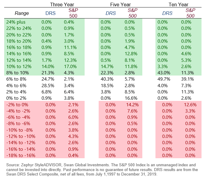
Compared to the S&P 500, the DRS Select Composite’s annualized five-year returns look very appealing.
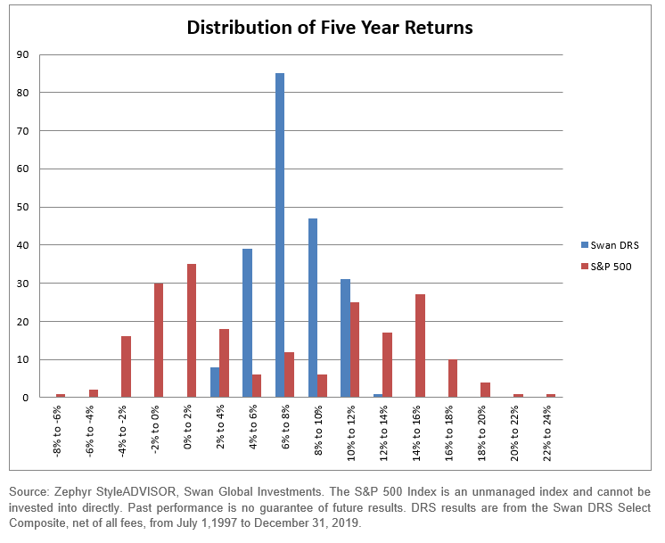
Almost two-thirds of the 211 observations occurred in the 6% to 10% range. The two most common buckets for the S&P 500 were the -2% to 0% and 0% to 2% ranges.
With a track record of over 20 years, the sample size affords a healthy number of decade-long returns to analyze—159 observations in all.
The long-term results of the DRS Select Composite show a remarkable degree of consistency. Again, the value of hedging against bear market losses is easily illustrated in this chart.
Return Consistency Addresses Investment Timing Risk
Another secondary, finer point of these charts has to do with timing.
At Swan we are often asked, “When is the best time to buy the DRS?” If an investor’s previous market experience has been in something like the S&P 500, it is a perfectly rational question to ask.
As we have seen, over the last 20 years one could have experienced radically different results, depending upon the time frame in question. However, the DRS Select Composite almost renders this question moot as the range of outcomes has been very tight, as seen in the next table:
As Mr. Griffey said, it’s important not to get too high or too low.